2-D Example

In this example, we run the HCT algorithm on the normalized Himmelblau objective. First, import all the functions needed

from PyXAB.synthetic_obj.Himmelblau import Himmelblau_Normalized        # the objective
from PyXAB.algos.HCT import HCT                                       # the algorithm
from PyXAB.partition.BinaryPartition import BinaryPartition             # the partition

# the other useful packages/functions
import numpy as np
from PyXAB.utils.plot import plot_regret

Define the number of rounds, the target, the domain, the partition, and the algorithm for the learning process

T = 1000                                                    # the number of rounds is 1000
target = Himmelblau_Normalized()                            # the objective to optimize is the normalized Himmelblau
domain = [[-5, 5], [-5, 5]]                                 # the domain is [[-5, 5], [-5, 5]]
partition = BinaryPartition                                 # the partition chosen is BinaryPartition
algo = HCT(domain=domain, partition=partition)              # the algorithm is HCT

To plot the regret, we can initialize the cumulative regret and the cumulative regret list

cumulative_regret = 0
cumulative_regret_list = []

In each iteration of the learning process, the algorithm calls the pull(t) function to obtain a point, and then the reward for the point is returned to the algorithm by calling receive_reward(t, reward). For a stochastic learning process, uniform noise is added to the reward.

for t in range(1, T+1):

    point = algo.pull(t)
    reward = target.f(point) + np.random.uniform(-0.1, 0.1)         # uniform noise
    algo.receive_reward(t, reward)

    # the following lines are for the regret
    inst_regret = target.fmax - target.f(point)
    cumulative_regret += inst_regret
    cumulative_regret_list.append(cumulative_regret)


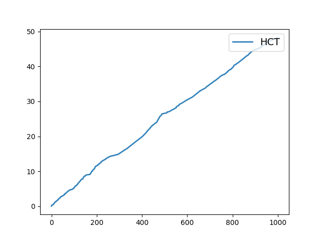
# plot the regret
plot_regret(np.array(cumulative_regret_list), name='HCT')

The following lines of code are only for creating thumbnails and do not need to be used

# sphinx_gallery_thumbnail_number = 2
import matplotlib.pyplot as plt
fig = plt.figure()
ax = fig.add_subplot(111, projection='3d')

x = np.linspace(domain[0][0], domain[0][1], 1000)
y = np.linspace(domain[0][0], domain[0][1], 1000)
xx, yy = np.meshgrid(x, y)
z = (- (xx ** 2 + yy - 11) ** 2 - (xx + yy ** 2 - 7) ** 2) / 890
ax.plot_surface(xx, yy, z, alpha=0.9)
fig.subplots_adjust(left=0.1, right=0.9, top=0.9, bottom=0.1)